Running a good simulation

It can be difficult to obtain well-equilibrated results for hard problems (such as the ferromagnet-spin-liquid transition on the pyrochlore lattice). It is therefore important to identify the problems in order to mitigate them.

Two sources of error

The algorithm has a systematic error coming from the finite projection depth. The projection depth is defined by step_size (denoted by \(\beta\) in the following) times the number of branching steps \(p\), divided by two:

\[\tau = \frac{p}{2}\,\beta\,.\]

\(\beta\) is an integer for the discrete methods and a floating-point number for the continuous-time method. The \(\tau\) values from the two methods should not be compared directly.
It further exhibits statistical errors coming from two origins. First, a finite number of measurements leads to statistical noise, which becomes problematic when the measurements are strongly autocorrelated. Second, the effective walker population collapses at large projection depth. After \(p\) branching steps, the entire population traces back to only a few ancestor configurations, or to a single one.

The effects of these errors become visible when the energy or an observable is tracked as a function of \(p\) over several independent runs. In a healthy simulation, every run converges to the same plateau, signaling that the projection has reached the ground state and that the statistical errors are small. If \(p\) is increased further, the plateau eventually deteriorates. There the algorithm fails because the population has collapsed to too few ancestors.

We illustrate the convergence for the critical spin-1/2 TFIM with \(N = 100\) sites (data of Fig. 4 of the paper). Each panel shows the difference to the exact value per site: energy (a), nearest-neighbor correlator (b), and transverse magnetization (c). Panel (c) is not measured separately: the energy is a linear combination of the correlator and the transverse magnetization, so (c) follows from (a) and (b).

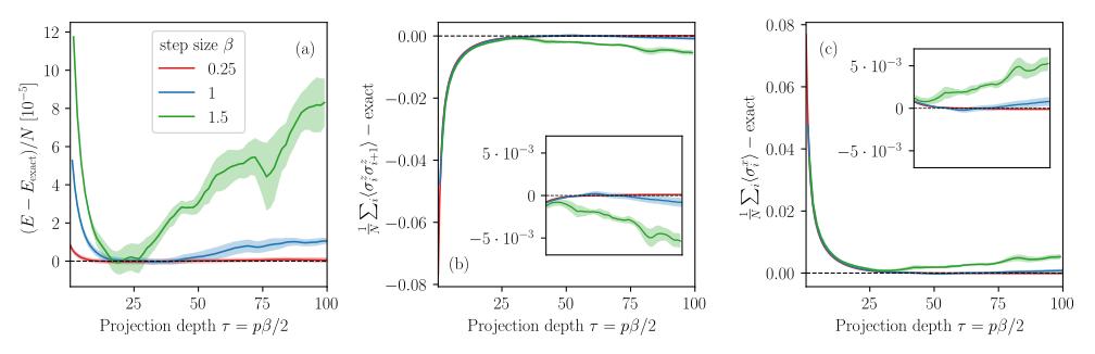
The figure shows data for three different step sizes, \(\beta = 0.25\) (red), \(\beta = 1\) (blue) and \(\beta = 1.5\) (green). \(\beta = 0.25\) is clearly superior, leading to a stable plateau for the entire projection depth of \(\tau=100\). The step size can be used to improve the convergence at larger projection depth. This is discussed in Tuning the step size. We find that the energy converges faster than the correlator and is more stable.

Finite projection depth

To check whether the projection depth is sufficient, track the observable of interest as a function of \(p\). If it settles on a plateau that is stable over several consecutive \(p\), the projection has converged. If it keeps moving, increase \(p\). Check each observable separately, as the energy usually converges at much smaller \(p\) than other observables. A better guiding wavefunction reduces the projection depth needed.

In the convergence figure above, the plateau is reached only for \(\tau \gtrsim 25\) for the observables.

Statistical errors

The most important error source is the collapse of the effective sample size, caused by the branching of walkers. A few lineages of ancestors (or a single one) dominate the reconfiguration and reduce the effective sample size. This collapse is why the plateau in the convergence figure deteriorates at large \(\tau\).

We define the effective sample size after \(m\) branching steps as

\[n_\mathrm{eff}(m) = \frac{N_\mathrm{walker}^2}{\sum_i c_i(m)^2} \in [1, N_\mathrm{walker}]\,,\]

where \(c_i\) is the number of walkers descending from the \(i\)-th initial walker after \(m\) steps. Note that an observable evaluated at \(p\) requires only \(m = p/2\) branching steps. We recommend \(n_\mathrm{eff} \gtrsim 50\) to get good statistics.

Every run reports the effective sample size in stats, at \(m = p/2\) for each window of p_array:

walkers, energy, obs, stats, raw = run(
    walkers, n_steps=2000, hamiltonian=H, step_size=0.2,
    guide=guide, p_array=[2, 4, 8, 16], rng_key=jax.random.PRNGKey(1),
    warmup_steps=1000, verbosity=0,
)
for m, n_eff in zip(stats["ancestor_m"], stats["effective_sample_size"]):
    print(f"p = {2 * int(m):3d}   n_eff = {n_eff:8.1f}")

It can also be computed using statistics(), without a production run, for any values in m_array:

from pygfmc import statistics

_, st = statistics(walkers, H, step_size=0.2, guide=guide, method="cont_time",
                   rng_key=jax.random.PRNGKey(7), m_array=[1, 5, 10, 20, 40],
                   quiet=True)
for m, n_eff in zip(st["ancestor_m"], st["effective_sample_size"]):
    print(f"m = {int(m):3d}   n_eff = {n_eff:8.1f}")

Another source of statistical noise is simply an insufficient number of measurements. While we recommend running independent Markov chains to identify this, evaluate_observables() provides the possibility to estimate the error bars of a single run with a blocked jackknife:

from pygfmc import evaluate_observables

E, O, E_err, O_err = evaluate_observables(raw, n_blocks=20)
for p in E:
    print(f"p = {p:3d}   E/L = {E[p] / L:.6f} +- {E_err[p] / L:.6f}")

Tuning the step size

Apart from a better guide and more walkers, the step size \(\beta\) is the most important knob for improving a calculation. To optimize it, choose a target projection depth \(\tau = p\beta/2\) and measure \(n_\mathrm{eff}\) as a function of \(\tau\) for several \(\beta\). The optimal \(\beta\) gives the largest \(n_\mathrm{eff}\) at the target \(\tau\):

import numpy as np
import matplotlib.pyplot as plt
from pygfmc import statistics

tau_max = 128.0                                      # target projection depth
betas   = [0.25, 0.5, 1, 2, 4, 8, 16, 32, 64, 128]  # step sizes to compare
seeds   = range(2)                                   # independent repetitions
colors  = plt.cm.viridis(np.linspace(0, 0.9, len(betas)))

fig, ax = plt.subplots(figsize=(6.5, 3.6))
for beta, color in zip(betas, colors):
    m_max   = round(tau_max / beta)
    m_array = np.unique(np.linspace(1, m_max, 32).round().astype(int))
    n_eff   = np.array([
        statistics(walkers, H, guide=guide,
                   avg_log_weight=stats["avg_log_weight"], step_size=beta,
                   method="cont_time", rng_key=jax.random.PRNGKey(seed),
                   m_array=m_array, quiet=True)[1]["effective_sample_size"]
        for seed in seeds])
    tau = m_array * beta                             # tau = (p/2) * beta = m * beta
    ax.errorbar(tau, n_eff.mean(axis=0),
                yerr=n_eff.std(axis=0, ddof=1) / np.sqrt(len(seeds)),
                fmt="o-", ms=4, capsize=2, color=color, label=f"{beta:g}")

ax.set_xlabel(r"Projection depth $\tau = p\beta/2$")
ax.set_ylabel(r"Effective sample size $n_\mathrm{eff}$")
ax.set_yscale("log")
ax.set_yticks([2**k for k in range(1, 11)], [str(2**k) for k in range(1, 11)])
ax.minorticks_off()
ax.set_xlim(0, tau_max)
ax.legend(title=r"step size $\beta$", loc="upper right", ncol=5)
fig.tight_layout()
fig.savefig("neff_vs_tau.pdf")

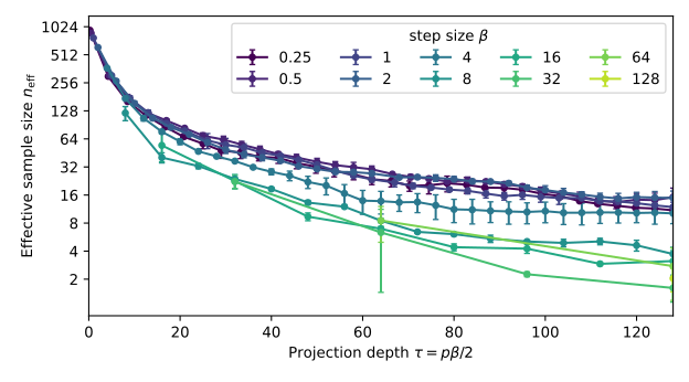
Effective sample size versus projection depth for ten step sizes

Step sizes from \(\beta = 0.25\) to \(2\) give nearly the same \(n_\mathrm{eff}\) up to \(\tau \approx 60\); at the largest depths \(\beta = 0.25\) and \(0.5\) keep slightly more. If multiple values lead to similarly good results, use the largest one for a shorter runtime.

Further tips

Equilibrate. Do an equilibration run first. The run function has the option to set warmup_steps.
Start in the right sector. If the Hamiltonian conserves a quantity, all walkers must be within the sector of interest (see Prepare walkers).
Use many walkers. The more walkers, the better.
Off-diagonal observables. Use off_diag_stride to reduce the autocorrelation time between measurements.
Discrete methods. If no diagonal element is present (e.g., pure hopping), we recommend working with the discrete method using method="single_step".
Check if a GPU is used:

python -c "import jax; print(jax.default_backend(), jax.devices())"

Invest in the guide

More walkers help, but a better guiding wavefunction is usually the more effective investment. See the kagome notebook.