Welcome to PyGFMC!
Python Green’s Function Monte Carlo (PyGFMC)
PyGFMC is a JAX-based implementation of Green’s Function Monte Carlo for ground states of sign-problem-free quantum lattice models. It
runs efficiently on GPUs,
provides access to diagonal and off-diagonal observables, and
accepts arbitrary variational wavefunctions as guides.
Install it from PyPI with pip:
pip install pygfmc               # GFMC only
pip install "pygfmc[netket]"     # + training guides with NetKet
What is Green’s Function Monte Carlo?
GFMC is a projection method on the ground state \(\vert\psi_0\rangle\) of a sign-problem-free Hamiltonian \(H\):
Evaluating this projection stochastically gives access to both diagonal and off-diagonal observables.
A key advantage compared to other Monte Carlo methods is the use of a guiding wavefunction, which is an approximation of the ground state that improves the sampling. The better the ansatz, the more effective the method becomes.
GPU acceleration
The JAX implementation provides GPU speedups of up to three orders of magnitude!
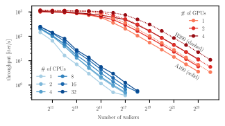
Throughput (iterations per second) versus the number of walkers on CPU cores and on A100 and H200 GPUs (Fig. 3 of the paper). The number of walkers sets the size of the simulation.
This speedup makes it possible to tackle problems that are extremely difficult to equilibrate! The figure below resolves the transition between the ferromagnet and quantum spin ice in the three-dimensional pyrochlore lattice:
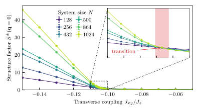
Transverse structure factor \(S^{\pm}(\mathbf{q}=0)\) of the nearest-neighbor pyrochlore XXZ model versus \(J_{xy}/J_z\) for system sizes up to \(N=1024\) (Fig. 6 of the paper). The transition sits at \(J_{xy}/J_z=-31/300\pm 1/1200\).
The setup
A PyGFMC simulation is built from four components:
a Hamiltonian,
an initial walker ensemble,
an optional guiding wavefunction, and
an optional set of observables to evaluate.
Running a simulation includes a step-by-step guide. See the Paper for more details and an explanation of the algorithm.
Quickstart
The example below simulates the Bose-Hubbard chain with at most two bosons per site,
guided by a Gutzwiller-Jastrow wavefunction,
where \(x_i\) is the occupation of site \(i\).
import jax
from pygfmc import run
from pygfmc.walkers import prepare_walkers_sz
from pygfmc.hamiltonian import BoseHubbard
from pygfmc.wavefunction import JastrowBoseHubbard, train_with_netket
import netket as nk

L       = 50
edges   = [[i, (i + 1) % L] for i in range(L)]   # periodic chain

H       = BoseHubbard.create(edges, t=1.0, eta=0.25, U=4.0, mu=1.0, n_max=2)
walkers = prepare_walkers_sz(512, L, jax.random.PRNGKey(0), sz=L, states=(0.0, 1.0, 2.0))

# variational optimization of beta, h and d with NetKet (stochastic reconfiguration)
guide   = JastrowBoseHubbard(L, edges, beta=0.0, h=0.0, d=0.5)
sampler = nk.sampler.MetropolisLocal(nk.hilbert.Fock(n_max=2, N=L))   # pair term: N not conserved
guide, history = train_with_netket(H, guide, sampler=sampler, n_iter=50, learning_rate=0.05,
                                   sr=True, qgt=nk.optimizer.qgt.QGTJacobianDense,
                                   return_history=True)
print(f"beta = {float(guide.beta[0]):.3f}, h = {float(guide.h[0]):.3f}, d = {float(guide.d[0]):.3f}")
print(f"variational energy per site: {history[-1] / L:.5f}")

walkers, energy, obs, stats, raw = run(
    walkers, n_steps=2000, hamiltonian=H, step_size=0.25,
    guide=guide, p_array=[8, 16, 32, 64], rng_key=jax.random.PRNGKey(1),
    warmup_steps=1000, verbosity=10
)

print({p: e / L for p, e in energy.items()})    # energy per site, DMRG: -2.026343